(LTT) Configure Source Model using class: Reflection_Source

XSPEC provides the xspec.models.Reflection_Source and xspec.models.Transmission_Source classes in order to provide an interpolation function over multiple source spectra simulations.

The reflection source spectrum as a function of source voltage and anode angles can be written as:

\[S^{sr}(E, v, \psi) = S^{sr}(E, v, \psi_0) \frac{Ph(E, v, \psi)}{Ph\left(E, v, \psi_0\right)}.\]

where:

• \(S^{sr}(E, v, \psi_0)\) is the interpolation function over a given list of spectra with different source voltages. It represents the source spectrum as a function of energy (\(E\)), source voltage (\(v\)), and a fixed anode angle (\(\psi_0\)), which serves as a reference.

• \(Ph(E, v, \psi)\) is the Philibert absorption correction factor, applied in an analytical model that considers the anode angle. This factor corrects for the absorption effects that are dependent on the anode angle (\(\psi\)).

Here is an example to configure the provided reflection source class. With the source spectra provided, configure the X-ray source by defining two continuous variables, voltages, and takeoff angle. The process involves two principal steps:

1. Configure the source model with Reflection_Source by passing two continuous parameters, voltages, and takeoff angle, which should be a tuple (init value, min, max). Note that setting min and max to None indicates that we do not need to optimize this parameter.

2. Reflection sources are an interpolation-based model. Use set_src_spec_list to set up a list of simulation source spectra with corresponding source voltages.

import numpy as np
import pyltt

def LTT_sim_source_sp(LTT, kV, takeOffAngle=11, anodeMaterial='W', energyBinSize=1, energyBinOffset=1):

    pyltt.reset(LTT, units='mm') #Use mm units for length

    LTT.run("takeOffAngle=%f"%takeOffAngle)
    LTT.run("simKV=%f"%kV)
    LTT.run("anodeMaterial=%s"%anodeMaterial)
    LTT.run("energyBinSize=%f"%energyBinSize)
    LTT.run("energyBinOffset=%f"%energyBinOffset)
    s_100 = LTT.getSpectrum()
    return  s_100

ltt_path = '/usr/workspace/prduePCI/LTT/IBM/python'
LTT = pyltt.ltt(ltt_path)


# Generate source spectra using Spekpy for a range of source voltages and a fixed takeoff angle.
min_simkV = 30
max_simkV = 200

simkV_list = np.linspace(min_simkV, max_simkV, 18, endpoint=True).astype('int')
reference_anode_angle = 11  # degrees
energies = np.linspace(1, max_simkV, max_simkV)  # energy range

src_spec_list = []
for simkV in simkV_list:
    # Creating a source spectrum array for each voltage
    src_spec = np.zeros((max_simkV))
    e,src_spec[:simkV] = LTT_sim_source_sp(LTT, simkV, reference_anode_angle)
    src_spec_list.append(src_spec)

from xspec.models import Reflection_Source
import matplotlib.pyplot as plt
import torch

# Initialize the Reflection_Source model with specified voltage and takeoff angle ranges.
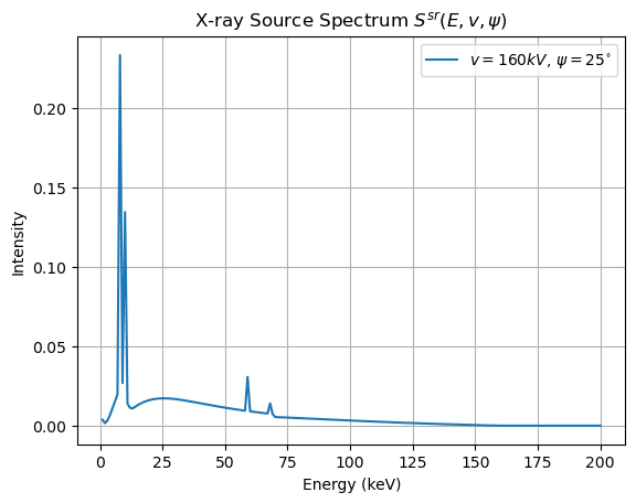
source = Reflection_Source(voltage=(160, 30, 200), takeoff_angle=(25, 5, 45), single_takeoff_angle=True)
source.set_src_spec_list(src_spec_list, simkV_list, reference_anode_angle)  # Set the source spectral list

# Plot the resulting spectrum without gradient descent modifications (torch.no_grad() context)
with torch.no_grad():
    plt.plot(energies, source(energies), label='$v=160 kV$, $\psi=25^{\circ}$')

plt.xlabel('Energy (keV)')  # X-axis label
plt.ylabel('Intensity')  # Y-axis label
plt.title('X-ray Source Spectrum $S^{sr}(E, v, \psi)$')  # Plot title
plt.legend()  # Add legend
plt.grid(True)  # Add grid for better readability
plt.show()  # Display the plot

# Initialize the Reflection_Source model with specified voltage and takeoff angle ranges.
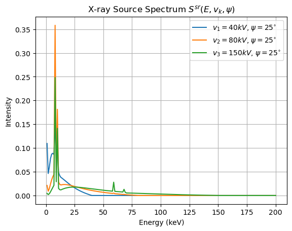
voltage_list = [40, 80, 150]
sources = [Reflection_Source(voltage=(v, 30, 200), takeoff_angle=(25, 5, 45), single_takeoff_angle=True) for v in voltage_list]
for si, source in enumerate(sources):
    source.set_src_spec_list(src_spec_list, simkV_list, reference_anode_angle)  # Set the source spectral list
    with torch.no_grad():
            plt.plot(energies, source(energies), label='$v_%d=%d kV$, $\psi=25^{\circ}$'%(si+1, voltage_list[si]))

plt.xlabel('Energy (keV)')  # X-axis label
plt.ylabel('Intensity')  # Y-axis label
plt.title('X-ray Source Spectrum $S^{sr}(E, v_k, \psi)$')  # Plot title
plt.legend()  # Add legend
plt.grid(True)  # Add grid for better readability
plt.show()  # Display the plot