Getting Started/Tutorial
Xspec aims to accurately determine the spectral response of X-ray systems by solving the inverse problem using calibration measurements.
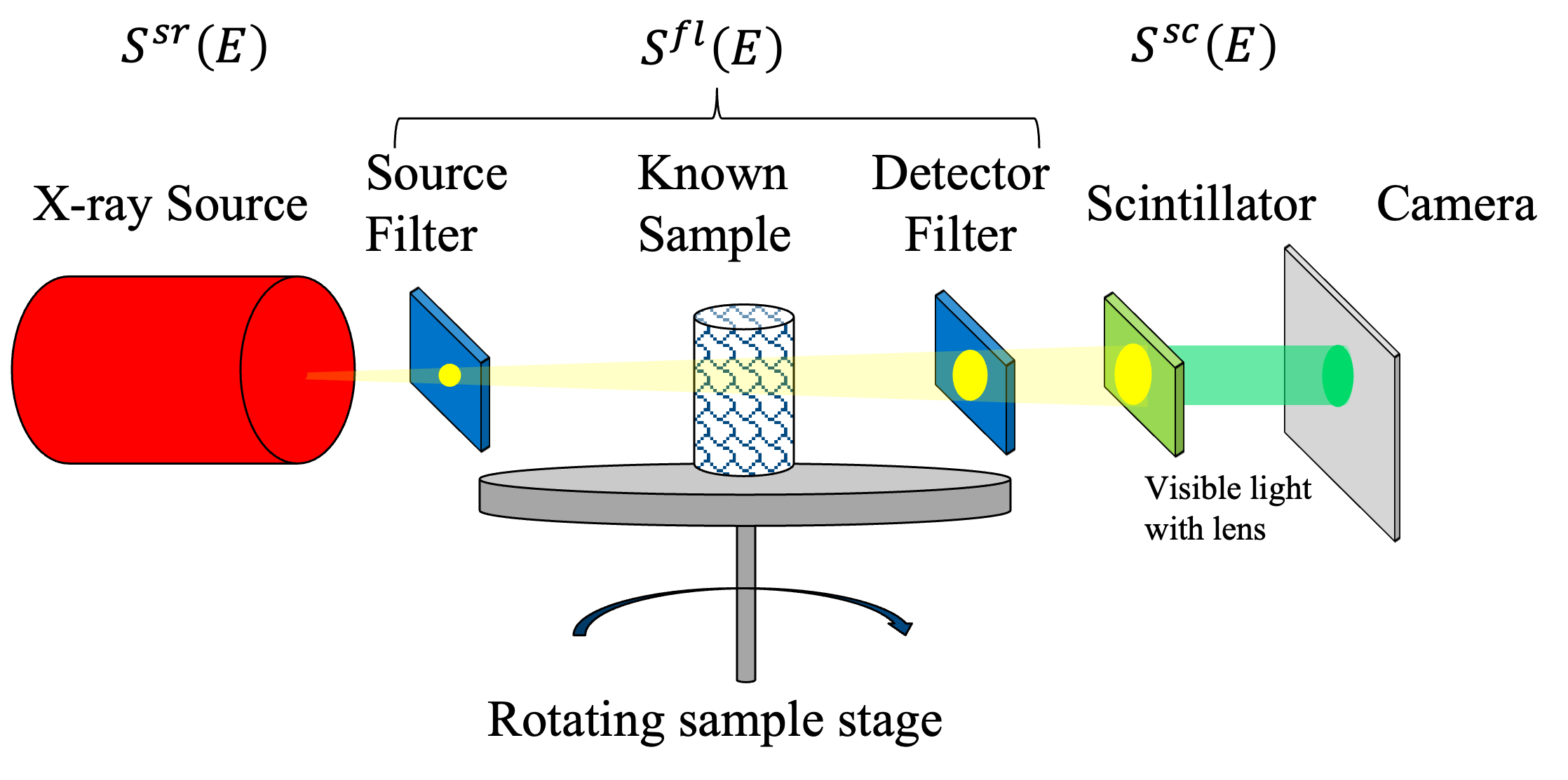
Physics model of CT scanning. A homogeneous cylindrical object is scanned. The total spectral response can be decomposed into the product of the X-ray source spectrum, filter response, and scintillator response, respectively.
Before reading the tutorial please prepare required information listed below
Normalized Radiograph: Users are required to provide a normalized radiograph for analysis.
System Components’ Information: Basic knowledge of the source, filter, and scintillator components used in the setup is necessary. This includes:
Source Types: Options include Transmission, Reflection, or Synchrotron, among others.
Possible Filter Materials
Possible Scintillator Materials
The specific component used in each measurement.
Homogeneous Samples with known composition and dimensions (Optional): Providing homogeneous samples, with their composition and dimensions known, is essential. If the user does not know the dimension of the sample, functions are provided to calibrate the dimension information from a 3D reconstruction.
0. Jupyter Notebooks Tutorials
The remainder of this tutorial outlines the steps involved in XSPEC’s spectral estimation with multiple jupyter notebook tutorials.
The [xspec] contains a number of example Python notebooks in the [examples] folder.
To run jupyter notebook:
If you install anaconda, in terminal, run
jupyter notebook
Access Kernel Menu: In the notebook toolbar, click on the “Kernel” menu to see a list of options.
Change Kernel: Select “Change kernel” from the dropdown. A list of available kernels will appear, including Python versions and any other kernels you have installed (like R, Julia, etc.).
Select Desired Kernel (xspec): Click on the kernel you wish to switch to. The notebook will refresh, and the new kernel will be activated.
Example Dependencies
Some examples use additional dependencies, which are listed in requirements.txt.
pip install -r demo/requirements.txt # Installs other example requirements
1. Total X-ray System Response
The total X-ray system response, \(S(E)\), describes the sensitivity across different energy bins, remaining constant when scanning various samples. This sensitivity is determined by the energy-wise product of three components: the source spectrum \(S^{sr}(E)\), the filter response \(S^{fl}(E)\), and the scintillator response \(S^{sc}(E)\):
We discretize the continuous functions \(S(E)\) by dividing them into \(N_j\) non-overlapping energy bins \([E_j, E_{j+1}]\). Thus, we define the discretized normalized spectral energy response value at the \(j^{th}\) energy bin as
The normalized X-ray System Response \(\mathbf{x}\) is one of essential knowledge we want to determine for further X-ray analysis.
Examples: Spectral Models
- The following Python notebooks teach you
How to utilize provided spectral classes to configure X-ray system components (source, filter, scintillator)?
How to customize your own spectral class to adapt to different scenarios?
2. Forward Modeling
In order to determine the spectral response of X-ray systems, we must link The normalized X-ray System Response \(x\), to the measurable data, \(y\). This connection is established through a model of the measurement process:
Forward modeling is a crucial step that allows us to predict how changes in \(\mathbf{x}\) affect our observed data, \(\mathbf{y}\). By comprehending this relationship, we can refine our measurements and enhance the accuracy of our spectral estimations.
How to get A?
Start from a single data point \(y\), which might pass through multiple homogenous samples.
Assuming that each LAC value of sample \(m\), \(\mu_m (E)\), is constant within each bin \(E \in [E_j, E_{j+1}]\), the total transmission of one scanning at the \(j^{th}\) energy bin is given by
where:
\(\Phi\) represents the material set, containing multiple homogenous materials;
\(L_{m}\) as the path length of the projection through the \(m^{th}\) material rod.
\(\mu_m(E)\) as the LAC of the material \(m\) at energy \(E\).
For 3 dimensional case, calculate the forward matrix(\(N_{\text{views}} \times N_{\text{rows}} \times N_{\text{cols}} \times N_E\)) using
the list of masks, LAC, and projector using xspec.calc_forward_matrix():
Examples: Forward Matrix
- The following Python notebooks teach you
How to obtain a list of masks from reconstructions?
How to configure your own forward projector (parallel beam, conebeam, fanbeam, etc.) to calculate the forward matrix?
3. Estimate System Parameters by Solving Inverse Problem
We define the MAP cost function for the multi-polychromatic dataset. This is accomplished by summing over all \(k\), as shown below:
where
\(\Theta\) denotes the aggregate set of parameters across all datasets, with \(K\) representing the total number of single-polychromatic datasets.
The parameter set \(\Theta\) is composed of the source parameters \(\left\{\theta_{a}^{sr} \mid a = 1, \ldots, N_a\right\}\), the filter parameters \(\left\{\theta_{b}^{fl} \mid b = 1, \ldots, N_b\right\}\), and the scintillator parameter \(\theta^{sc}\).
\(\Lambda^{(k)}\) can be identity matrix or diagonal matrix with \(\Lambda_{i, i}^{(k)}=\frac{1}{y_i}\).
The optimal parameter set \(\Theta^*\) is determined by minimizing \(L(\Theta)\) using gradient descent:
where \(\mathcal{U}\) represents the constrained solution space.
Examples: Spectral Estimation
- The following Python notebooks teach you
How to generate a simulated dataset?
How to do spectral estimation with prepared spectral models and forward matrices?